Introduction. I—Leads, rate, rhythm, and cardiac axis
BMJ 2002; 324 doi: https://doi.org/10.1136/bmj.324.7334.415 (Published 16 February 2002) Cite this as: BMJ 2002;324:415
- Steve Meek,
- Francis Morris
Electrocardiography is a fundamental part of cardiovascular assessment. It is an essential tool for investigating cardiac arrhythmias and is also useful in diagnosing cardiac disorders such as myocardial infarction. Familiarity with the wide range of patterns seen in the electrocardiograms of normal subjects and an understanding of the effects of non-cardiac disorders on the trace are prerequisites to accurate interpretation.

The contraction and relaxation of cardiac muscle results from the depolarisation and repolarisation of myocardial cells. These electrical changes are recorded via electrodes placed on the limbs and chest wall and are transcribed on to graph paper to produce an electrocardiogram (commonly known as an ECG).
The sinoatrial node acts as a natural pacemaker and initiates atrial depolarisation. The impulse is propagated to the ventricles by the atrioventricular node and spreads in a coordinated fashion throughout the ventricles via the specialised conducting tissue of the His-Purkinje system. Thus, after delay in the atrioventricular mode, atrial contraction is followed by rapid and coordinated contraction of the ventricles.
The electrocardiogram is recorded on to standard paper travelling at a rate of 25 mm/s. The paper is divided into large squares, each measuring 5 mm wide and equivalent to 0.2 s. Each large square is five small squares in width, and each small square is 1 mm wide and equivalent to 0.04 s.
Throughout this article the duration of waveforms will be expressed as 0.04 s = 1 mm = 1 small square
The electrical activity detected by the electrocardiogram machine is measured in millivolts. Machines are calibrated so that a signal with an amplitude of 1 mV moves the recording stylus vertically 1 cm. Throughout this text, the amplitude of waveforms will be expressed as: 0.1 mV = 1 mm = 1 small square.

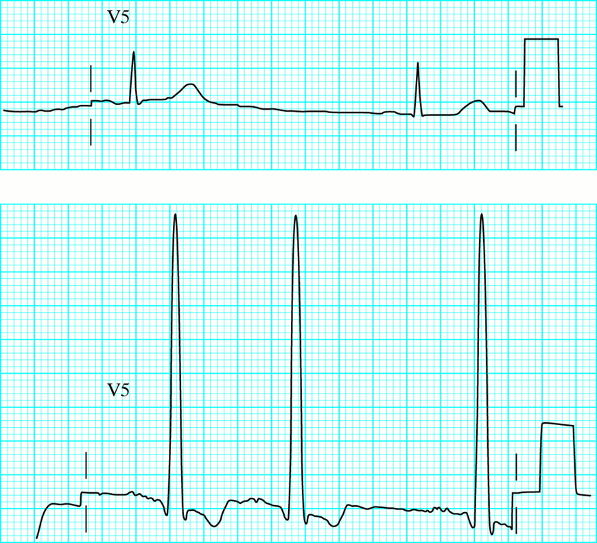
Role of body habitus and disease on the amplitude of the QRS complex. Top: Low amplitude complexes in an obese woman with hypothyroidism. Bottom: High amplitude complexes in a hypertensive man
The amplitude of the waveform recorded in any lead may be influenced by the myocardial mass, the net vector of depolarisation, the thickness and properties of the intervening tissues, and the distance between the electrode and the myocardium. Patients with ventricular hypertrophy have a relatively large myocardial mass and are therefore likely to have high amplitude waveforms. In the presence of pericardial fluid, pulmonary emphysema, or obesity, there is increased resistance to current flow, and thus waveform amplitude is reduced.
The direction of the deflection on the electrocardiogram depends on whether the electrical impulse is travelling towards or away from a detecting electrode. By convention, an electrical impulse travelling directly towards the electrode produces an upright (“positive”) deflection relative to the isoelectric baseline, whereas an impulse moving directly away from an electrode produces a downward (“negative”) deflection relative to the baseline. When the wave of depolarisation is at right angles to the lead, an equiphasic deflection is produced.

Wave of depolarisation. Shape of QRS complex in any lead depends on orientation of that lead to vector of depolarisation
The six chest leads (V1 to V6) “view” the heart in the horizontal plane. The information from the limb electrodes is combined to produce the six limb leads (I, II, III, aVR, aVL, and aVF), which view the heart in the vertical plane. The information from these 12 leads is combined to form a standard electrocardiogram.

Position of the six chest electrodes for standard 12 lead electrocardiography. V1: right sternal edge, 4th intercostal space; V2: left sternal edge, 4th intercostal space; V3: between V2 and V4; V4: mid-clavicular line, 5th space; V5: anterior axillary line, horizontally in line with V4; V6: mid-axillary line, horizontally in line with V4
The arrangement of the leads produces the following anatomical relationships: leads II, III, and aVF view the inferior surface of the heart; leads V1 to V4 view the anterior surface; leads I, aVL, V5, and V6 view the lateral surface; and leads V1 and aVR look through the right atrium directly into the cavity of the left ventricle.
Anatomical relations of leads in a standard 12 lead electrocardiogram
II, III, and aVF: inferior surface of the heart
V1 to V4: anterior surface
I, aVL, V5, and V6: lateral surface
V1 and aVR: right atrium and cavity of left ventricle

Vertical and horizontal perspective of the leads. The limb leads “view” the heart in the vertical plane and the chest leads in the horizontal plane
Rate
The term tachycardia is used to describe a heart rate greater than 100 beats/min. A bradycardia is defined as a rate less than 60 beats/min (or <50 beats/min during sleep).
One large square of recording paper is equivalent to 0.2 seconds; there are five large squares per second and 300 per minute. Thus when the rhythm is regular and the paper speed is running at the standard rate of 25 mm/s, the heart rate can be calculated by counting the number of large squares between two consecutive R waves, and dividing this number into 300. Alternatively, the number of small squares between two consecutive R waves may be divided into 1500.
Waveforms mentioned in this article (for example, QRS complex, R wave, P wave) are explained in the next article
Some countries use a paper speed of 50 mm/s as standard; the heart rate is calculated by dividing the number of large squares between R waves into 600, or the number of small squares into 3000.

Regular rhythm: the R-R interval is two large squares. The rate is 150 beats/min (300/2=150)
“Rate rulers” are sometimes used to calculate heart rate; these are used to measure two or three consecutive R-R intervals, of which the average is expressed as the rate equivalent.
When using a rate ruler, take care to use the correct scale according to paper speed (25 or 50 mm/s); count the correct numbers of beats (for example, two or three); and restrict the technique to regular rhythms.
When an irregular rhythm is present, the heart rate may be calculated from the rhythm strip (see next section). It takes one second to record 2.5 cm of trace. The heart rate per minute can be calculated by counting the number of intervals between QRS complexes in 10 seconds (namely, 25 cm of recording paper) and multiplying by six.

A standard rhythm strip is 25 cm long (that is, 10 seconds). The rate in this strip (showing an irregular rhythm with 21 intervals) is therefore 126 beats/min (6×21). Scale is slightly reduced here
Rhythm
To assess the cardiac rhythm accurately, a prolonged recording from one lead is used to provide a rhythm strip. Lead II, which usually gives a good view of the P wave, is most commonly used to record the rhythm strip.
Cardinal features of sinus rhythm
The P wave is upright in leads I and II
Each P wave is usually followed by a QRS complex
The heart rate is 60-99 beats/min
The term “sinus rhythm” is used when the rhythm originates in the sinus node and conducts to the ventricles.
Young, athletic people may display various other rhythms, particularly during sleep. Sinus arrhythmia is the variation in the heart rate that occurs during inspiration and expiration. There is “beat to beat” variation in the R-R interval, the rate increasing with inspiration. It is a vagally mediated response to the increased volume of blood returning to the heart during inspiration.
Normal findings in healthy individuals
Tall R waves
Prominent U waves
ST segment elevation (high-take off, benign early repolarisation)
Exaggerated sinus arrhythmia
Sinus bradycardia
Wandering atrial pacemaker
Wenckebach phenomenon
Junctional rhythm
1st degree heart block
Cardiac axis
The cardiac axis refers to the mean direction of the wave of ventricular depolarisation in the vertical plane, measured from a zero reference point. The zero reference point looks at the heart from the same viewpoint as lead I. An axis lying above this line is given a negative number, and an axis lying below the line is given a positive number. Theoretically, the cardiac axis may lie anywhere between 180 and −180°. The normal range for the cardiac axis is between −30° and 90°. An axis lying beyond −30° is termed left axis deviation, whereas an axis >90° is termed right axis deviation.

Hexaxial diagram (projection of six leads in vertical plane) showing each lead's view of the heart
Conditions for which determination of the axis is helpful in diagnosis
Conduction defects—for example, left anterior hemiblock
Ventricular enlargement—for example, right ventricular hypertrophy
Broad complex tachycardia—for example, bizarre axis suggestive of ventricular origin
Congenital heart disease—for example, atrial septal defects
Pre-excited conduction—for example, Wolff-Parkinson-White syndrome
Pulmonary embolus
Several methods can be used to calculate the cardiac axis, though occasionally it can prove extremely difficult to determine. The simplest method is by inspection of leads I, II, and III.
Calculating the cardiac axis
Calculating the cardiac axis

Determination of cardiac axis using the hexaxial diagram (see previous page). Lead II (60°) is almost equiphasic and therefore the axis lies at 90° to this lead (that is 150° to the right or −30° to the left). Examination of the adjacent leads (leads I and III) shows that lead I is positive. The cardiac axis therefore lies at about −30°
A more accurate estimate of the axis can be achieved if all six limb leads are examined. The hexaxial diagram shows each lead's view of the heart in the vertical plane. The direction of current flow is towards leads with a positive deflection, away from leads with a negative deflection, and at 90° to a lead with an equiphasic QRS complex. The axis is determined as follows:
Choose the limb lead closest to being equiphasic. The axis lies about 90° to the right or left of this lead
With reference to the hexaxial diagram, inspect the QRS complexes in the leads adjacent to the equiphasic lead. If the lead to the left side is positive, then the axis is 90° to the equiphasic lead towards the left. If the lead to the right side is positive, then the axis is 90° to the equiphasic lead towards the right.
Steve Meek is consultant in emergency medicine at the Royal United Hospitals, Bath.
Footnotes
The ABC of clinical electrocardiography is edited by Francis Morris, consultant in emergency medicine at the Northern General Hospital, Sheffield; June Edhouse, consultant in emergency medicine, Stepping Hill Hospital, Stockport; William J Brady, associate professor, programme director, and vice chair, department of emergency medicine, University of Virginia, Charlottesville, VA, USA; and John Camm, professor of clinical cardiology, St George's Hospital Medical School, London. The series will be published as a book in the summer.