Article Text

Statistics from Altmetric.com
Objectives
-
Dealing with paired parametric data
-
Comparing confidence intervals and p values
In covering these objectives the following terms will be introduced:
-
Parametric and non-parametric analysis
-
Paired z test
-
Paired t test
We have shown previously that statistical inference enables general conclusions to be drawn from specific data. For example estimating a population's mean from a sample mean. At first glance this may not appear important. In practice however the ability to make these estimations is fundamental to most medical investigations. These tend to concentrate on dealing with one or more of the following questions:
Have the observations changed with time and/or intervention?
Do two or more groups of observations differ from each other?
Is there an association between different observations?
To answer these questions many different types of statistical inference tests have been developed to deal with varying sample sizes and different types of data. Though the tests differ they have the common aim of assessing whether the null hypothesis is likely to be correct (box 1). They are known collectively as “tests of significance”.1
Box 1 The null hypothesis
There is no difference between the groups with respect to the measurement made.
The significance test chosen is dependent upon the type of data we are dealing with, whether it has a normal distribution and the type of question being asked.2 Once the distribution of the data is known, you can tell if the null hypothesis should be tested using parametric or non-parametric methods.
Parametric and non-parametric analysis
PARAMETRIC ANALYSIS
A normal distribution is a regular shape. As such it is possible to draw the curve exactly by simply knowing the mean, standard deviation and variance of the data. When considering a normal distribution of a population these features are known as parameters. Parametric analysis relies on the data being normally (or nearly) distributed so that an estimation of the underlying population's parameters can be made.3 These can then be used to test the null hypothesis. As only quantitative data can have a normal distribution, it follows that parametric analysis can only be used on quantitative data (table 1).
Types of test of significance for two group comparison
Key point
All parametric tests use quantitative data but not all quantitative data have to be analysed using parametric tests.
NON-PARAMETRIC ANALYSIS
These tests of the null hypothesis do not assume any particular distribution for the data. Instead they look at the category or rank order of the values and ignore the absolute difference between them. Consequently non-parametric analysis is used on nominal and ordinal data as well as quantitative data that are not normally (or nearly normally) distributed (table 1).
If a difference exists between the study groups, it is more likely to be found using parametric tests. It is therefore important to know for certain if the data are normally distributed. You can sometimes determine this by checking the distribution curve of the plotted data. A more formal way is to use a computer to show how precisely the data fit with a normal distribution. This will be described in greater detail in the next article. When data are not normally distributed attempts are often made to transform it so that parametric analysis can be carried out. The commonest method used is logarithmic transformation.2 This has the added advantage of allowing geometric means and confidence intervals to be calculated that have the same units as the original data.
Key points
-
Non-parametric analysis can be used on any data but parametric analysis can only be used when the data are normally distributed.
-
Provided they are appropriately used, parametric tests derive more information about the whole population than non-parametric ones.
Having determined that parametric analysis is appropriate you then need to select the best statistical test. This depends upon the size of the samples and the type of question being asked. In all cases however the following systematic approach is used (box 2).
Box 2 System for statistical comparison of two groups
-
State the null hypothesis and the alternative hypothesis of the study
-
Select the level of significance
-
Establish the critical values
-
Select a sample and calculate its mean and standard error of the mean (SEM)*
-
Calculate the test statistic
-
Compare the calculated test statistic with the critical values
-
Express the chances of obtaining results at least this extreme if the null hypothesis is true
Paired or independent parametric analysis
Two types of parametric statistical tests can be used to compare the means of two study groups. The choice depends upon whether the data you are dealing with are independent or paired.
Data can be considered to be paired when two related observations are taken with analysis concentrating on the difference between the paired scores. Examples of these type of data include:
-
“Before” and “after” studies carried out on the same subjects
-
Observations made on individually matched pairs where only the factor under investigation is different
Independent data are when the subjects for the two groups are picked at random such that selection for one group will not effect the subjects chosen for the other. The tests used to analyse these data will be discussed in the next article. For now we will concentrate on paired data.
PAIRED TESTS
Both z and t tests can be used to investigate the difference between the means of two sets of paired observations. The former is, however, only valid if the samples are sufficiently large.4 When this is not the case we can use the t statistic provided that the population of the mean differences in scores between the pairs is approximately normally distributed.4 As this is often the case the paired t test, rather than its z counterpart, is more commonly seen in the medical literature. To show how these tests are applied consider the following examples.
PAIRED Z TEST
Dr Egbert Everard continues to work in the Emergency Department of Deathstar General. His consultant, Dr Canute, asks him to find out if Neverwheeze, the new bronchodilator for asthmatics, significantly changes patient's peak flow rate (PFR). To do this he follows the systematic approach described in box 2.
1 State the null hypothesis and alternative hypothesis of the study
Having considered the problem, Egbert writes down the null hypothesis as:
“There is no difference in asthmatic patient's PFR before and after receiving Neverwheeze”.
This can be summarised to:
Mean difference in PFR = 0
The alternative hypothesis is the logical opposite of this, that is:
“There is a difference in asthmatic patient's PFR before and after receiving Neverwheeze”.
This can be summarised to:
Mean difference in PFR ≠ 0
2 Select the level of significance
If the null hypothesis is correct the PFR before and after Neverwheeze should be the same. However, even if this were true it would be very unlikely they would be exactly the same because of random variation between patients. You would expect some PFR to increase and others to fall. Overall however the mean difference between the two groups should be zero if the null hypothesis is valid.
When groups are widely separated it is likely that the null hypothesis is not valid. For example, if 100 people died in your department one day and none the next then its highly unlikely that a difference this big would be attributable to chance. In contrast you would be less confident to rule out the effect of chance if the difference in death rate was only 1. The question therefore is how big does the difference need to be before the null hypothesis can be rejected?
Rather than guessing, it is better to consider what values are possible. If we measured the mean PFR difference in groups of asthmatic patients selected randomly we would find the sample means form a normal distribution around the population's mean difference. As it is a normal distribution it is possible to convert this to a standard normal distribution.5 The probability of getting a particular sample mean can then be read from the table of z statistics where:
z = [sample mean difference −population mean difference (μ)]/standard error of the mean (SEM)
Where:
SEM = population standard deviation (σ)/√number in the sample (n)
In this case we do not know the value of σ. Nevertheless, provided the sample size is large enough (that is, greater than or equal to 100) the z statistic can still be used.4 This relies on the fact that a valid estimation of the population's standard deviation can be derived from the sample data (s).4
Key point
Provided the sample is ≥ 100:
SEM = ESEM = s/√n
By convention, the outer 0.025 probabilities (that is, the tips of the two tails representing 2.5% of the area under the curve) are considered to be sufficiently away from the population mean as to represent values that cannot be simply attributed to chance variation (fig 1). Consequently, if the sample mean is found to lie in either of these two tails then the null hypothesis is rejected. Conversely, if the sample mean lies within these two extremes then the null hypothesis will be accepted (fig 1). In doing this we are accepting that normal samples that fall into these two tails will be incorrectly labelled as being abnormal. Therefore a total of 5% of all possible sample means from the normal population will incorrectly reject the null hypothesis.1

Random sampling distribution of mean differences for a hypothetical population. μhyp = mean of the hypothetical population. Zcrit = critical value of z separating the areas of acceptance and rejection of the null hypothesis.
Following convention, Egbert picks a significance level of 0.05 for his study. He now needs to determine the PFR that demarcates this level of probability. These are known as the critical values.
3 Establish the critical values
Using the z table Egbert finds that the critical value (zCRIT) demarcating the middle 95% of the distribution curve is z = +/− 1.96 (fig 1). In other words a z value of +/− 1.96 separates the middle 95% area of acceptance of the null hypothesis from two 2.5% areas of rejection.
With the null and alternative hypotheses defined, and the critical values established (zCRIT), the patients for the study can now be selected. The z statistic derived from the sample (zCALC) can then be determined.
Key point
The z test is when you compare zCRIT and zCALC
4 Study a sample and calculate its mean
With the critical values known, Edgar now gathers a sample of 100 patients and measures the PFR. Following Neverwheeze he finds the mean PFR increases by 5 l/minute and s is 20 l/minute.
5 Calculate the test statistic
As explained before the z statistic is equal to:
z = [sample mean difference − population mean difference (μ)]/ESEM
Where ESEM equals s/√n
Therefore: ESEM = 20/10 = 2
According to the null hypothesis the mean difference for the population is zero, consequently:
z statistic = 5−0/2 = 2.5
In other words the mean difference before and after using Neverwheeze lies 2.5 ESEM above the population's mean difference of zero.
6 Compare the calculated test statistic with the critical values
The calculated value of +2.5 lies above the larger critical value of 1.96. It therefore falls into the area of rejecting the null hypothesis.
7 Express the chances of obtaining results at least this extreme if the null hypothesis is true
The p value is the probability of getting a mean difference equal to or greater than that found in the experiment, if the null hypothesis was correct.1 As the z value can be negative or positive, there are two ways of getting a difference with a magnitude of 2.5. Consequently the p value is represented by the area demarcated by −2.5 to the tip of the left tail plus the area demarcated by +2.5 to the tip of the right tail (fig 1).
From the z statistic table Egbert finds the probability of getting a difference equal to, or greater than, +2.5 is 0.5−0.4938 = 0.0062. Similarly, getting a difference equal to, or greater than, −2.5 is also 0.0062. In total therefore there is only a 0.0124 chance (1.2%) that a difference of 2.5 ESEM could be produce if the null hypothesis was correct.
Consequently Egbert can tell Dr Canute that “The hypothesis that there is no difference in the PFR before and after Neverwheeze is rejected. The mean difference = 5 l/minute, p = 0.012”.
Key points
-
The z distribution tables can be used to convert the z statistic into a p value.
-
The p value represents the chances of getting an experimental result this big, or greater, if the null hypothesis applied.
In days gone by the analysis would stop at this point. Nowadays it is usual practice to also consider the confidence interval of the results whenever possible. Before carrying out these calculations it is pertinent to consider why the confidence intervals are considered so useful.
Confidence intervals and p values
As demonstrated in the previous example statistical inference can be used to produce a p value for the mean difference. The latter is known as the point (or sample) estimate along with a p value. In contrast, a confidence interval (CI) around the point estimate provides a range within which the value of the particular parameter would lie if the whole population was considered.4 For example, a 95% confidence interval around a study's mean difference is the range of values the population's mean difference could be expected to be found 95% of the time. This is a similar part to that played by the standard error of the mean (SEM).5 In these cases the 95% confidence interval is equal to the sample mean +/− 1.96 SEM.
To help understand the importance of this, consider a trial of two antihypertensives, A and B. This study found that the group taking drug A had a mean systolic blood pressure that was 40 mm Hg less than group B (p = 0.0001). The low p value indicates the result is statistically significant and the large point estimate implies the finding is clinically relevant. However, if you repeated this study using similar, but different groups of patients, then the magnitude of the blood pressure change would vary. The CI allows you to work out how wide this variation is likely to be. In this study the 95%CI was 32.0 to 49.0 mm Hg. Consequently the mean blood pressure fall for 95% of the whole population of similar hypertensives lies between 32 and 49 mm Hg. Even at the lower end of the spectrum this is a sizable reduction and therefore likely to be clinically useful if the side effects and costs are similar with both treatments.
It is important to bear in mind that although we are 95% confident that the true value lies within the range provided, it does not mean it has an equal chance of lying anywhere along the CI. In actual fact the probability varies, with the most likely value being that calculated originally. Therefore, using the example above, the most likely reduction in blood pressure for all similar hypertensives is 40 mm Hg but in 95% of cases it could vary between 32 and 49 mm Hg.
Key points
-
The point estimate is the best guess for the true difference based upon the study's results
-
The CI is the range of possible values of the point estimate
Though the 95% CI is often chosen, the actual level is up to that which you consider the most appropriate. For example, you can use CI of 99.9% when the treatment is potentially harmful or very expensive. The effect is to widen the range of values covering the point estimate to ensure the widest range of possible differences is identified.
Key point
The choice of CI is a balance between ensuring the population mean is included while minimising parts of the scale where it is unlikely to be.
The confidence interval also provides information on the precision of the study—that is, the ability to determine the true value for the whole population. If the 95% CI in a similar study, involving two hypotensives C and D, was −5.0 to 50 mm Hg then it could be that Group C did worse than D (that is, the difference = −5.0 mm Hg) or did very much better (that is, the difference = 50 mm Hg). Equally the true difference could lie anywhere between these two extremes. Wide intervals around the point estimate indicate the study lacks precision. Usually this is due to there being too few subjects in the experiment.
Key point
Generally, confidence intervals decrease with increases in sample size
The above example also shows that a confidence interval can include 0. When this occurs it means there is a chance there is no difference between the study groups. This is the same as having a p value greater than 0.05 (or your chosen significant level) and not rejecting the null hypothesis. Consequently the CI can provide all the information available from a p value. In addition it tells you the suitability of rejecting or accepting the null hypothesis.
Key point
A negative result (that is, accept the null hypothesis) occurs when the confidence interval includes zero or only clinically irrelevant difference between the groups
In summary therefore, confidence intervals provide information on:
-
The magnitude of the difference
-
The precision of the study
-
The statistical significance
Key point
As p values imply little about the magnitude and precision of the differences between the groups, CI should be reported instead.
Confidence intervals are worked out on a computer using a set of mathematical rules. However, the method used to calculate them needs to take into account the type of data and the study design. Advice is therefore recommended in choosing the most appropriate type of CI calculation. Furthermore, although confidence intervals are an excellent way of summarising information, they cannot control for other errors in study design such as improper patient selection and poor experimental methodology. For example, a small CI obtained from a biased study is less likely to include the true population value than one that is unbiased. Consequently the narrow CI gives a false impression of precision.
In view of the importance of confidence intervals, Egbert now wants to determine the 95% CI for the mean difference.
As described in the previous article,4 the 95% CI is:
Where zo is the z statistic appropriate to the required CI. Consequently the 95% confidence interval of the difference is:

As this range does not include zero, Egbert concludes that data are not compatible with the null hypothesis being correct. However, the range of PFR covers small values. Therefore rather than simply presenting a p value Egbert will be able to provide more information if he uses the 95% confidence interval when discussing the clinical relevance of these data.
A lot of information has been presented over the last few paragraphs. It is therefore useful to take a moment to re-read the basic system for comparing two groups statistically (box 2). This is used, with slight variations, in the majority of situations you will come across because it applies equally to comparing means, proportions, slopes of lines and many other common statistical analyses.
Paired t test
If the sample size in the example above was smaller than 100 then a paired t test would have to be used. To demonstrate this, consider the following case.
Egbert informs Dr Endora Lonely about his findings regarding Neverwheeze. She is surprised because they use a lot of it in the Emergency Department at St Heartsinc where she works as a SpR. She therefore decides to repeat the study using 25 patients attending her department.
1 State the null hypothesis and alternative hypothesis of the study
These remain the same. Consequently:
The null hypothesis can be summarised to:
Mean difference in PFR = 0
And the alternative is:
Mean difference in PFR ≠ 0
2 Select the level of significance
Following convention, Endora picks a significance level of 0.05 for her study.
3 Establish the critical values
It is not possible to calculate the SEM when the standard deviation of the population is not known, or the sample size is less than 100. In these cases the t statistic has to be used instead of the z statistic.4
As described in the previous article, the t tables use degrees of freedom rather than the number in the group.4 This is equal to one less than the group size. Consequently Endora looks up the value for t with a significance of 0.05 and 24 degrees of freedom (fig 2). This is the critical value (tCRIT) and in this case is equal to 2.064. In other words, for a sample size of 25, a t value of +/− 2.064 separates the middle 95% area of acceptance of the null hypothesis from two 2.5% areas of rejection.
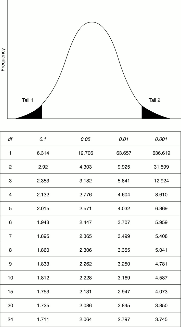
Extract of the table of the t statistic values. The first column lists the degrees of freedom (df). The headings of the other columns give probabilities for t to lie within the two tails of the distribution.
As with the z test, the t statistic derived from the sample (tCALC) can now be determined.
Key point
The t test is when you compare tCRIT and tCALC
4 Study a random sample and calculate its mean
With the critical values known, Endora can now carry out her study. Following Neverwheeze she finds the mean PFR increases by 81 l/minute and s is 135 l/minute.
5 Calculate the test statistic
As explained in a previous article the t statistic is equal to5:
[study's mean difference − population's mean difference]/ESEM
where ESEM equals s/√n
Therefore: ESEM = 135/5 = 27
Consequently:
In other words the mean difference before and after using Neverwheeze lies 3 ESEM above the population's mean difference of zero.
6 Compare the calculated test statistic with the critical values
The calculated value of +3 lies above the larger critical value of 2.064. It therefore falls into the area of rejecting the null hypothesis.
7 Express the chances of obtaining results at least this extreme if the null hypothesis is true
As the t value can be negative or positive, there are two ways of getting a difference with a magnitude of 3. Consequently the p value is represented by the area demarcated by −3 to the tip of the left tail plus the area demarcated by +3 to the tip of the right tail.
Endora finds that for 24 degrees of freedom, this t value for the sum of these two tails corresponds to a probability between 0.001 (0.1%) and 0.01 (1.0%). There is therefore only a 0.001–0.01 chance that a difference of 3 ESEM could be produce if the null hypothesis was correct.
Consequently Endora can claim that “The hypothesis that there is no difference in the PFR before and after Breatheeze is rejected, t = 3.0, df 24, p < 0.01”.
Key point
The t distribution table can be used to convert the t statistic into a p value
Endora now wants to determine the 95% CI for the mean difference.
As described previously,4 the 95% CI is:
Where to is the t statistic appropriate to the required CI. For a sample size of 25 (df = 24) this is 2.064. Consequently the 95% confidence interval of the difference is:
As this range does not include zero, she concludes that data are not compatible with the null hypothesis being correct. However, the range of PFR again includes small values. The 95% confidence interval is therefore helpful when discussing the clinical relevance of these data.
Summary
Carrying out comparisons of two groups is helped greatly by having a systematic approach. In this way the null hypothesis will be defined and the type of data identified. An appropriate test can then by chosen and a computer program used, or a preset recipe followed, until the answer is produced.
When using the z test, the system for statistical comparison is followed using the z value for the test statistic and tables derived from the standard normal distribution. Similarly, when using the t test, the system for statistical comparison is followed using the t value for the test statistic and tables derived from the t distribution. In practice the t test is more commonly used because there are more situations in which it is more appropriate.
Probabilities are used in statistical inference studies that are assessing the validity of the null hypothesis. Though a simple p value can be listed, confidence intervals provide the point estimate (that is, size of the possible differences) and the precision of the result. For most clinical studies confidence intervals are therefore more relevant than p values.
Quiz
-
What is the systematic method of comparing two groups?
-
What are the requirements of the data if parametric analysis is to be carried out?
-
What is the recommended sample size for carrying out a paired z test?
-
The following example is adapted from the study by Guy et al.6 Their aim was to assess the physiological responses in rats to a primary blast. Using nine matched pairs they compared the respiratory rate following an abdominal shock wave with the control group. Five minutes after the blast the difference in respiratory rate was 15 breaths/ minute with s equal to 4.5 breaths/ minute. What is the 95% confidence interval for this difference?
-
One for you to try on your own. Sisley et al carried out a study to assess the performance of doctors in ultrasound evaluation.7 As part of this study they tested the factual knowledge of 33 emergency physicians before and after tuition. They found the improvement to be 39.2 with s equal to 1.7. What is the 95% CI for this difference?
Answers
-
See box 2
-
It needs to be normally (or nearly normally) distributed
-
Greater than, or equal to, 100
-
The 95% CI is:
mean difference +/− [to × ESEM]
For a sample size of nine (df = 8) to is 2.262. The ESEM is s/√n. Consequently the 95% confidence interval of the difference is:
15 +/− [2.262 × 4.5/3]
=12–18 breaths/minute (rounded up to the nearest whole number)
Further reading
-
Altman D. Theoretical distributions. In: Practical statistics for medical research. London: Chapman Hall, 1991:48–73.
-
Altman D. Comparing groups—continuous data. In: Practical statistics for medical research. London: Chapman Hall, 1991:179–228.
-
Bland M. An introduction to medical statistics. Oxford: Oxford University Press, 1987.
-
Gaddis G, Gaddis M. Introduction to biostatistics: Part 4, statistical inference techniques in hypothesis testing. Ann Emerg Med 1990;19:820–5.
-
Gardner M, Altman D. Calculating confidence intervals for means and their differences. In: Statistics with confidence. London: BMJ, 1989:20–7.
-
Glaser A. Hypothesis testing. In: High yield biostatistics. Baltimore: Williams and Wilkins, 1995:31–46.
-
Koosis D. Difference between means. In: Statistics—a self teaching guide. 4th ed. New York: Wiley, 1997:27–152.
-
Normal G, Steiner D. Comparing the mean of 2 samples: the t test. In: PDQ statistics. St Louis: Mosby, 1997:37–42.
-
Swincow T. The t test. In: Statistics from square one. London: BMJ, 1983:33–42.
Acknowledgments
The authors would like to thank Sally Hollis, Jim Wardrope and Iram Butt for their invaluable suggestions.