Article Text

Statistics from Altmetric.com
Objectives
-
Estimating an element from a population with known standard deviation
-
Estimating a statistic from a population with known standard deviation
In covering these objectives we will introduce the following terms:
-
Standard normal distribution
-
z statistic
-
Confidence intervals
In the previous article the term inferential statistic was introduced.1 This form of numeric manipulation is often used to estimate a population's parameter from a sample's statistic. For example, inferential statistics would be used to estimate a population's mean from a sample's mean. It can also be used to do the opposite—that is, estimate a sample statistic from a population's parameter. This is not commonly done because it requires the population's mean and standard deviation to be known and this is rarely the case.
In both calculations the values obtained are only estimations because of the normal variation that occurs. We can however work out the probability of a particular value based upon information from either the sample or population. Central to this is converting the original data to a standard normal distribution so that these estimations can be made.
Standard normal distribution
A standard normal distribution is a particular type of normal distribution that has the following properties:
-
Symmetrical bell shaped curve
-
Mean equal to zero
-
Standard deviation equal to 1
-
Total area under the curve equal to 1
It is possible to convert any normal distribution to a standard normal distribution by adjusting it such that the population mean becomes zero and the standard deviation is equal to 1. To do this, each of the data points (elements) is modified by:
-
Subtracting the population mean
-
Dividing the result by the standard deviation of the population
The final value is known as the z statistic. The z statistic is therefore describing the size of the difference between the element (X) and population's mean (μ) value in multiples of the population's standard deviation (σ). For example, a z statistic of +1.5 means the difference between the element and mean value is +1.5 times the size of the standard deviation of the population.
Key points
-
It is possible to convert any normal distribution to a standard normal distribution
-
The Greek letters μ and σ are often used to respectively represent the population's mean and standard deviation
-
Therefore for any element the z statistic is equal to [X−μ]/σ
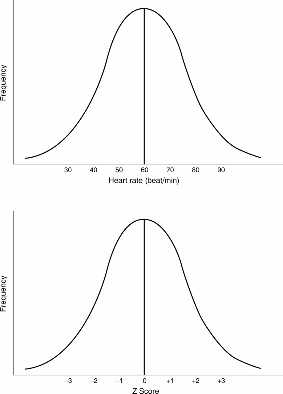
When a normal distribution is plotted as a standard normal distribution, the original values on the horizontal axis are converted to their equivalent z statistic. To demonstrate this consider the continuing work of Egbert Everard in the Emergency Department of Deathstar General. Following his previous work, he suspects that the men in the department could be unfit. He therefore decides to explore this further by looking at the resting heart rate. He finds in a physiology textbook that resting heart rate for fit men (μ) is 60/min with a standard deviation (σ) of 10 (fig 1). Two of the staff members he finds are Charge Nurse “Pot belly” Pete the hospital's darts and wine tasting expert and “Skier” Sphen the locum SHO from Sweden. They have resting heart rates of 90 and 40/min respectively.

Normal distribution of resting heart rate in fit men and standard normal distribution using the same data.
Consequently the z statistic for “Pot belly” Pete's resting heart rate is:
90–60/10 = 3
and the z statistic for “Skier” Sphen's resting heart rate is:
40–60/10 = −2
Plotting these on a standard normal distribution curve, “Pot belly”'s result lies three standard deviations above the mean of fit men whereas Sphen lies two standard deviations below (fig 2).

Standard normal distribution of resting heart rate along with “Pot belly” Pete and “Skier” Sphen's results.
Key points
-
The z statistic is the number of standard deviations an element is from the mean
-
A positive z statistic indicates an element value greater than the mean
-
A negative z statistic indicates the value of the element is less than the mean
The above examples show that it is possible to convert a normal distribution to a standard distribution by altering the value of the element to a z statistic. This is important because z statistic tables can then be used to estimate the probability of the particular value occurring. These tables show a column for the z value adjacent to the corresponding area under the distribution curve between the mean and the z point (fig 3).

Extract of a table of z scores. An entry in the table is the proportion under a standard normal distribution curve from z = 0 to a positive value of z (for example, z = 3). Areas for the negative z values are obtained by symmetry. The curve accompanies the table to show which areas were used to derive the z values.
For example a z value of +1.96 demarcates 47.5% of the area under the curve. This extends from the midline to a vertical line drawn through +1.96 on the horizontal axis (fig 4 (A)). Therefore the total proportion to the left of this z value equals 0.5 + 0.475 = 0.975 (97.5%). This is because each half of the curve represents a proportion of 0.5 (50% of the area under the curve). Consequently the chances of getting a z value of +1.96 (or less) is 97.5%.

Standard normal distribution showing two ways of calculating areas for the same value of z.
Figure 3 lists proportions for the right half of the curve. However, as the standard normal distribution is symmetrical, the right and left halves are equal. Therefore the area under the curve between the midline and −1.96 is also 47.5%. Be aware also that some z tables give the area from the particular z value to the tip of the tail (fig 4(B)). Tables therefore either have a description or a diagram on the top to ensure you are reading them correctly (fig 3).
Key points
-
A standard normal distribution is important because the proportion under the curve demarcated by any value of z has already been calculated and is available in z statistic tables.
-
If the numerical value of z and −z are equal, the proportions (percentage of the area under the curve) are the same but in opposite directions.
-
Z statistic tables can differ in which the area under the curve is described
It follows that by changing to a standard normal distribution it is possible to determine:
-
The probability of getting an element greater than or equal to a particular value
-
The range of element values that have a particular probability of occurring
-
The probability of getting an element between two particular values.
We now need to consider how these probabilities can be calculated when we are dealing with three different situations (box 1).
Box 1 Three common estimations
-
A single value from a population with known μ and σ
-
A sample mean from a population with known μ and σ
-
A sample mean from a population with unknown μ and σ
This article will deal with the first two situations. The third scenario will be dealt with in article 5 of this series.
Estimating a single value from a population with known μ and σ
THE CHANCE OF GETTING AN ELEMENT GREATER THAN OR EQUAL TO A PARTICULAR VALUE
Consider “Pot belly” Pete, what would be the chance of getting a resting heart rate equal or greater than 90 and still be part of the fit male population?
Using the z statistic tables (fig 3), the area demarcated by z = 0 (that is, the mean) and z = 3 is 0.4987.
The area under the curve represents the total probability and is equal to 1.0. As the curve is symmetrical, the area under each half is 0.5. Consequently the probability of getting a value greater than or equal to 3.0 is represented by area under the curve to the right of the shaded area. This is:
0.5–0.4987 = 0.0013.
Therefore the chances of being a fit man and having a resting heart rate greater than or equal to 90/min is 0.0013 or 0.13%.
THE RANGE OF ELEMENT VALUES WITH A PARTICULAR PROBABILITY OF OCCURRING
Following on from this result Egbert considered the right side of the distribution curve showing the resting heart rates of fit men. He wanted to know the resting heart rate that separated the upper 2.5% of the population from the remaining 97.5%. This is determined by carrying out the reverse of the method described above.
-
Convert the percentage to a proportion by dividing by 100.
2.5% is 0.025 when expressed as a proportion.
-
Determine the proportion of a standard normal distribution curve from the midline to 0.025.
Using figure 4(B) as a reference, it can be seen that the answer is equal to:
0.5–0.025 = 0.475
-
Convert the proportion 0.475 to a z statistic.
Using the z statistic tables, 0.475 gives a z statistic of 1.96 (fig 3).
-
Using this value for z, determine the element value.
Remembering that:
z = [Element value−Population mean]/Population standard deviation
1.96 = [Element value−60]/10
Therefore the element value is 19.6 + 60 = 80/min (rounded up)
Consequently the top 2.5% of the population of fit men have a resting heart rate of approximately 80/min or greater.
THE CHANCE OF GETTING AN ELEMENT BETWEEN TWO PARTICULAR VALUES
Egbert has often seen in published work, ranges of values for the middle 95% of the population. He therefore would like to know what is the range of resting heart rates of the middle 95% of the population of fit men. Looking at figure 5, you can see the middle 95% leaves two tails each representing 2.5% of the area under the curve (fig 5).
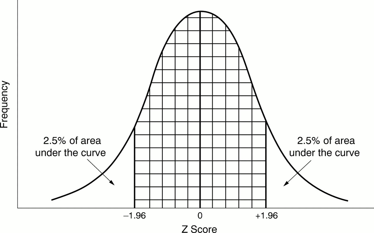
Standard normal distribution showing two 2.5% tails.
The value demarcating the upper 2.5% has already been calculated (that is, 80/min). Therefore Egbert only has to repeat the procedure for the lower 2.5%.
-
Convert the percentage to a proportion by dividing by 100.
2.5% is 0.025 when expressed as a proportion
-
Determine the proportion of a standard normal distribution curve from the midline to 0.025.
This is equal to:
0.025–0.5 = −0.475. The negative value indicates we are dealing with the left side of the curve.
-
Convert the proportion −0.475 to a z statistic.
Using the z statistic tables, −0.475 gives a z statistic of −1.96 (fig 3).
-
Using this value for z, determine the element value.
−1.96 = Element value−60/10
Consequently the element value is −19.6 + 60 = 40/min (rounded down). In other words the lower 2.5% of the population of fit men have a resting heart rate of approximately 40/min or less. Egbert therefore concludes that the middle 95% range is from approximately 40 to 80/min.
To check if you are confident with these calculations, take a moment to fill in the gaps in table 1 (answers on page 415).
Practising with z statistics
Key points
-
It is possible to convert elements in a normal distribution to a z statistic so that they can be plotted on a standard normal distribution
-
This conversion allows the probability of the element occurring to be determined
It is pertinent to notice at this time that the middle 95% of the population is represented by the mean +/− 1.96 standard deviations. This is usually rounded up to the mean +/− 2 standard deviations. Using this same system it is possible to calculate the percentage of the area of the curve covered by various standard deviations on either side of the mean (table 2). You can now see how, in article 2, the percentages of the area under the curve were derived.2
Percentage of the normal distribution
Another way of calculating the percentage (or proportion) of the area between two z statistics is to subtract the area under the curve to the left of the smaller z value from the larger one (fig 5). For example, the area to the left of a z statistic equal to −1.96 is 0.025 (2.5%). Conversely the area to the left of z of 1.96 is 0.5 + 0.475 (97.5%). Consequently, the probability of a value lying between these two z statistics is:
0.975−0.025 = 0.95 (95%)
Estimating a sample mean from a population with known μ and σ
To tackle this problem we need to remind ourselves about the properties of the standard error of the mean (SEM). In article 2 we described how normally distributed data from a sample could be summarised by recording the mean and standard deviation.2 We also went on to show how it is possible to use the mean calculated from a particular study (called the sample mean) to estimate the overall mean (called the population mean). Samples selected randomly from the same population are unlikely to have exactly the same means. This is attributable to chance variation and is known as random error. The SEM quantifies this by indicating the range, above and below the sample mean, in which the population mean lies. Another factor affecting the SEM is the size of the sample from which it is estimated. As sample size increases, the SEM variation caused by random error decreases.
Key point
SEM = Population standard deviation (σ)/number in the sample (n)
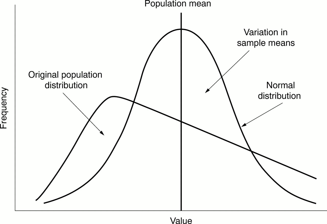
It can be shown that if random samples are taken, which are sufficiently large, their mean will form a normal distribution irrespective of the original population's distribution (fig 6). Furthermore, if an infinite number of samples were taken, the mean of the distribution and population would be the same. The mathematical proof for these statements comes from the central limit theorem.

Skewed original population with a normal distribution of sample means around the population mean.
For obvious reasons we cannot take such a large number of samples. Nevertheless we can use the SEM to estimate the limits within which the population mean will lie. As the distribution is normal, there is a 95% chance that the population's mean will lie somewhere between 1.96 × SEM below the sample mean to 1.96 × SEM above the sample mean.
Key points
-
The SEM is a measure of the deviation of sample means from the population mean
-
The accuracy of the SEM is dependent upon the samples being representative of the population and being randomly selected
-
The size of the SEM is dependent upon the size and variability of the sample
-
As the sample size increases, the SEM will get smaller and there will be closer agreement between the sample and population means
To help demonstrate these points consider the following hypothetical example. Suppose you wanted to find the mean presenting peak expiratory flow rate (PEFR) for adult asthmatic patients attending your emergency department. If you took the measurements in a sample of 20 patients you could work out the mean for that sample. However, if you then repeated this process in another 20 patients you would not expect exactly the same value. This is because of the chance variation between patients. Nevertheless if you continued to carry on making these recordings in more samples of similar size you would find eventually that there would be a normal distribution of the sample means. The central limit theorem indicates that the overall mean of these samples would be the same as the population mean. The standard deviation of this normal distribution is called the SEM. Consequently 95% of samples of adult asthmatic patients attending your emergency department will have a mean presenting PEFR lying between the population's mean value +/− 2 SEM.
In summary therefore when a large number of randomly selected and representative sample means are plotted they take on a normal distribution with the mean being the population mean and the standard deviation being the SEM. It is therefore possible to convert this distribution to a standard normal type so that you can determine:
-
The chance of getting a sample mean greater than or equal to a particular value
-
The range of a sample means with a particular chance of occurring
-
The chance of getting a sample mean between two particular values
THE CHANCE OF GETTING A SAMPLE MEAN GREATER THAN OR EQUAL TO A PARTICULAR VALUE
To demonstrate this, consider Egbert's result when he has measured the resting heart rate in all of the 25 male members of the department. He finds that the sample mean is 67/min and wants to know what would be the chance of getting a resting heart rate equal or greater to this and still be part of a normal fit male population?
The z statistic for this resting heart rate is:
[Sample mean−Population mean]/SEM
Where:
SEM = Population standard deviation (σ)/size of the sample (n)
Therefore in this case:
SEM = 10/√25 = 2.0
Therefore the z statistic is:
[67−60]/2.0 = +3.5
Using the z statistic table, the area between z = 0 and z = +3.5 is 0.4989. Therefore the probability of getting a z value greater than or equal to 3.5 is:
0.5−0.4989 = 0.0011
Consequently the chances of a similar sample of fit men having a resting heart rate greater than or equal to 67/min is 0.0011 or 0.11%.
THE VALUE OF SAMPLE MEAN WITH A PARTICULAR CHANCE OF OCCURRING
As before Egbert then turns his attention to the right tail of the distribution of mean values. Assuming a sample consists of 25 fit men who have been randomly selected, Egbert wants to know what sample mean demarcates the upper 2.5% of the population. This is carried out in a similar manner to that used when an element was considered.
-
Convert the 2.5% to the proportion 0.025
-
Determine the proportion of a standard normal distribution curve from the midline to 0.025. This is equal to 0.5−0.025 = 0.475
-
Convert the proportion 0.475 to a z statistic.
Using the z statistic tables, 0.475 gives a z statistic of 1.96 (fig 3).
-
Using this value for z, determine the sample mean.
Remembering that:
z = [Sample mean−Population mean]/SEM
1.96 = [Sample mean−60]/2
Therefore the element value is 3.92 + 60 = 64/ min (rounded up). Consequently 2.5% of these samples that have been randomly selected would have a mean resting heart rate of 64/min or greater.
THE CHANCE OF GETTING A SAMPLE MEAN BETWEEN TWO PARTICULAR VALUES
Looking at the middle of the distribution, Egbert then wants to know what range of means from similar samples demarcate the middle 95% of the population.
As the upper 2.5% has already been calculated (64/min), Egbert calculates the value for the lower 2.5%. Using the same system as before he works out that the proportion of a standard normal distribution curve from the midline to 0.025 is:
0.025−0.5 = −0.475
He then uses the z statistic tables to convert the proportion −0.475 to a z statistic and finds this to be −1.96 (fig 3).
Using this value for z, the sample mean can be determined by:
−1.96 = [Sample mean−60]/2
Therefore the element value is −3.92 + 60 = 56/min (rounded up).
Consequently the middle 95% of random samples of 25 fit men would have a mean resting heart rate between 56 and 64/min.
As with the situation with elements and standard deviations, we can see that the middle 95% of all the sample means is represented by the population mean +/− 1.96 standard errors of the mean. This is usually rounded up to the mean +/− 2 SEM. Using this same system it is possible to determine the percentage of the area of the curve covered by various multiples of the SEM on either side of the mean (table 3).
Percentage of the normal distribution
Answer to table 1 : practising with z statistics
From the calculations carried out above, we know that 95% of all sample means will lie within approximately 2 SEM of the population mean. In other words knowing the population mean, we can calculate the range in which the sample means will lie 95% of the time. For example, if the population mean is 50 cm with a SEM of 5 cm, 95% of all sample means will lie between:
[Mean−2 × SEM] to [Mean + 2 × SEM]
This is equal to:
[50−10] to [50 + 10] = 40 cm−60 cm
At first glance this may not seem very useful because we usually do not know the population mean. However if the 95% of the sample means are within 2 SEM of the population mean, it follows that the population mean lies within 2 SEM of a sample mean 95% of the time. For example, if the mean of a randomly selected sample is found to be 120 mm Hg and the SEM known to be 6, there is a 95% chance that the true population mean lies between:
Mean [+/− 2 SEM] = 120 [+/− 12] = 108 to 132 mm Hg
This range of values is known as the 95% confidence interval. In other words we are 95% confident that population's mean lies between 108 and 132 mm Hg.
Generally the confidence interval range is equal to the sample mean plus/minus [z statistic obtained from the z table for the required percentage level of confidence (zo)] multiplied by the SEM]. As an equation:
In this way we do not need to measure every single blood pressure in a particular population. Instead the sample is used to make an estimation of the range of possible values. In considering this range it is important to bear in mind that the best single estimation of the population's mean is the sample mean.
Key point
In general the CI is equal to sample mean +/− [z × SEM]. Where the z statistic is appropriate to the level of confidence you require. As 95% CI are often used this is approximately equal to the sample mean +/− [2 SEM].
Now that you have seen how CI are derived you will appreciate the range is dependent upon the SEM. As the latter is equal to the σ/n, the range can only be reduced by increasing the sample size. However, the range is proportional to the square root of the sample size. Consequently increasing the sample size by fourfold will only halve the confidence interval.
Summary
It is possible to convert a normal distribution to a standard type. This enables you to use the z statistic table to calculate the proportion of particular areas under the distribution curve. If the population's mean and standard deviation are known, it is possible to estimate:
-
The probability of getting an element or statistic greater than or equal to a particular value
-
The value of an element or statistic with a particular probability of occurring
-
The probability of getting an element or statistic between two particular values.
In addition, the latter range can be used to determine the confidence intervals for the estimated values.
Quiz
-
Assuming a standard normal distribution, what is the probability of a value being:
Greater than, or equal to, 2 standard deviations above the mean?
Less than, or equal to, 1.5 standard deviations below the mean?
Between 3 standard deviations below the mean to 1 standard deviation above it?
-
Assuming a standard normal distribution, what is the value of X if you are told that the probability of having this figure, or greater, is 0.15 (that is, 15%)?
-
What is the probability of getting a Hb concentration of 16.0 g, or higher, if the Hb distribution is normal and has a mean of 15.0 g with a standard deviation of 0.3?
-
Assume that a previous study has shown that the mean presenting PEFR for asthmatic men attending your emergency department is 685 l/min with a standard deviation of 30 l/min. What are the chances of a sample of 36 asthmatic men having a mean PEFR of 700 l/min?
-
In another department the mean presenting PEFR in a sample of women is found to be 400 l/min with a SEM of 20 l/min. What is the best single estimation of the population mean and what is its 95% confidence intervals?
Answers
-
Assuming a standard normal distribution, the probability of a value being:
Greater than, or equal to, 2 standard deviations above the mean is 0.5−0.4772 = 0.0228
Less than, or equal to, 1.5 standard deviations below the mean is 0.4332 + 0.5 = 0.9332
Between −3 standard deviations and +1 standard deviation from the mean is 0.4987 + 0.3413 = 0.84
-
If the probability of getting a value an element value (X), or greater, is 0.15, the probability of a value less than this is 0.85. As this standard normal distribution the area under the curve from this value to the mean is 0.85−0.5 = 0.35. The z statistic for 0.35 is 1.04.
We know that:
z statistic = [X − μ]/σ
Therefore:
X = 1.04 [σ] + μ
Assuming a standard normal distribution, σ equals 1 and μ zero, X equals 1.04.
-
We know that:
z statistic = [X − μ]/σ
Therefore:
z statistic = [16−15]/0.3
Therefore a Hb of 16 g is 3.3 standard deviations from the mean. The normal distribution tables show that the area to the left of this point is 0.999. Therefore the probability of getting a value of 16 g or higher is 1−0.999 = 0.001 (that is, one in a thousand).
-
z = Sample mean−Population mean (μ)/SEM
SEM = Population standard deviation (σ)/√n = 30/6 = 5
Therefore:
z = 700−685/5 = 3.
Using the z table, a z score of 3 corresponds to a probability of 0.4987. Therefore the chances of a sample having a mean PEFR of 700 l/min, or greater is 0.5−0.4987 = 0.0013 (that is, just over one in a thousand).
-
The best single estimation comes from the sample mean—that is, 400l/min.
The 95% confidence intervals = Sample mean +/− 1.96 × SEM
Therefore the 95% CI = 400 +/− 1.96 × 20 = 361−439 l/min.
Further reading
-
Bowyers D. Measuring spread. In: Statistics from scratch. Chichester: Wiley, 1996:114–49.
-
Glaser A. Descriptive statistics. In: High yield statistics. Baltimore: William and Wilkins, 1995:1–18.
-
Glaser A. Inferential statistics. In: High yield statistics. Baltimore: William and Wilkins, 1995:9–30.
-
Koosis D. Populations and samples. In: Statistics—a self teaching guide. 4th ed. New York: Wiley, 1997:40–76.
-
Norman G, Streiner D. Statistical inference. In: PDQ statistics. 2nd ed. St Louis: Mosby, 1997:17–36.
Acknowledgments
The authors would like to thank Sally Hollis, Jim Wardrope and Iram Butt for their invaluable suggestions.
References
Linked Articles
- Correction